3. A quickstart example

In this page we show how to use galario in some typical use cases, e.g. the fit of some interferometric data sets.

galario has been designed to simplify and accelerate the task of computing the synthetic visibilities given a model image, leaving to the user the freedom to choose the most appropriate statistical tool for the parameter space exploration.

For the purpose of these examples we will adopt a Bayesian approach, using Monte Carlo Markov chains to explore the parameter space and to produce a sampling of the posterior probability function. In particular, we will use the MCMC implementation in the emcee Python package.

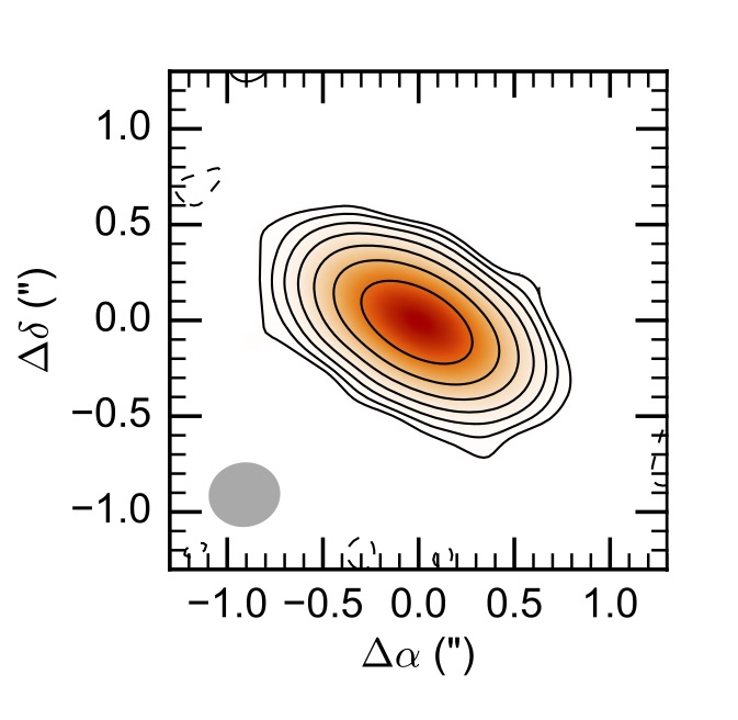
In this page we will show how to fit the mock observations of a protoplanetary disk. In particular, in the example we will analyse mock visibilities of the disk continuum emission at \(\lambda=\) 1 mm whose synthetized map is shown in this figure:

You can download here an ASCII version of the uv-table used in this example.

---

3.1. Fit a single-wavelength data set

1) Import the uv table

First, let’s import the table containing the interferometric observations. Typically, an interferometric data set can be exported to a table containing the \((u_j, v_j)\) coordinates (\(j=1...M\)), the Real and Imaginary part of the complex visibilities \(V_{obs\ j}\), and their theoretical weight \(w_{j}\), for example:

u  [m]          v  [m]          Re  [Jy]        Im  [Jy]        w
-------------------------------------------------------------------------
-155.90093      234.34887        0.01810         0.13799        200.05723
9.290660        362.97853       -0.05827         0.02820        216.95405
95.23531        109.22704        0.06314        -0.16727        167.18789
94.01319        251.97293        0.01974         0.04358        179.69114
-60.45751       211.33346        0.14856        -0.07756        188.09953
91.59843        68.94947         0.12741        -0.12871        156.32432
23.29531        251.71338        0.01568        -0.12316        189.58017
-135.83509      -29.77982       -0.02017        -0.00010        207.29354
59.38624        144.99431        0.04759        -0.08606        201.32301
192.43093       171.57617       -0.02176        -0.02661        208.52030
-243.91416      76.18790        -0.02306        -0.01430        207.16036
58.72442        276.64959        0.03325         0.04560        173.15922
35.56591        111.28235        0.03777        -0.11856        194.83899
...             ...             ...             ...             ...

You can download here an ASCII version of the uv-table used in this example.

A table like this one can be read with:

u, v, Re, Im, w = np.require(np.loadtxt("uvtable.txt", unpack=True), requirements='C')
wle = 1e-3  # [m]
u /= wle
v /= wle

where the \(u_j\) and \(v_j\) coordinates have been converted in units of the observing wavelength, 1 mm in this example. The np.require command is necessary to ensure that the arrays are C-contiguous as required by galario (see FAQ 1.1).

2) Determine the image size

Once imported the uv table, we can start using galario to compute the optimal image size

from galario.double import get_image_size

nxy, dxy = get_image_size(u, v, verbose=True)

where the returned values are the number of pixels (nxy) and the pixel size (dxy) in radians. nxy and dxy are chosen to fulfil criteria that ensure a correct computation of the synthetic visibilities. For more details, refer to Sect. 3.2 in Tazzari, Beaujean and Testi (2018) MNRAS 476 4527.

3) Define the brightness model

Let us define the model: for this example, we will use a very simple Gaussian profile:

from galario import arcsec

def GaussianProfile(f0, sigma, Rmin, dR, nR):
    """ Gaussian brightness profile. """

    # radial grid
    R = np.linspace(Rmin, Rmin + dR*nR, nR, endpoint=False)

    return f0 * np.exp(-0.5*(R/sigma)**2)

where f0 (Jy/sr) is a normalization, sigma is the width of the Gaussian, Rmin is the innermost radius of the grid, dR is the size of radial grid and nR is the number of radial grid cells. sigma, Rmin, dR should be passed to GaussianProfile() in arcseconds and f0 in Jy/sr.

4) Setup the MCMC Ensemble Sampler

In our fit we will have 6 free parameters: on top of the model parameters f0 and sigma we want to fit the inclination inc, the position angle PA, and the angular offsets \((\Delta RA, \Delta Dec)\) with respect to the phase center. Following the notation of the emcee documentation, we initialise the EnsembleSampler

from emcee import EnsembleSampler

# radial grid parameters
Rmin = 1e-4  # arcsec
dR = 0.01    # arcsec
nR = 2000

# parameter space domain
p_ranges = [[1, 20],
            [0., 8.],
            [0., 90.],
            [0., 180.],
            [-2., 2.],
            [-2., 2.]]

ndim = len(p_ranges)        # number of dimensions
nwalkers = 40               # number of walkers

nthreads = 4                # CPU threads that emcee should use

sampler = EnsembleSampler(nwalkers, ndim, lnpostfn,
                          args=[p_ranges, Rmin, dR, nR, nxy, dxy, u, v, Re, Im, w],
                          threads=nthreads)

where:

• p_ranges is a rectangular domain in the parameter space that defines the search region;

• lnpostfn is the posterior probability function;

• args defines an array of fixed parameters that lnpostfn takes additionally in input.

5) Define the posterior and the prior probability functions

Let us now implement the posterior function, using galario to compute the \(\chi^2\). Since in this example we are assuming an axisymmetric brightness profile we will use the chi2Profile function, but the same design holds for the chi2Image function that should be used for non-axisymmetric profiles.

from galario import deg, arcsec
from galario.double import chi2Profile

def lnpostfn(p, p_ranges, Rmin, dR, nR, nxy, dxy, u, v, Re, Im, w):
    """ Log of posterior probability function """

    lnprior = lnpriorfn(p, p_ranges)  # apply prior
    if not np.isfinite(lnprior):
        return -np.inf

    # unpack the parameters
    f0, sigma, inc, PA, dRA, dDec = p

    f0 = 10.**f0        # convert from log to real space

    # convert to radians
    sigma *= arcsec
    Rmin *= arcsec
    dR *= arcsec
    inc *= deg
    PA *= deg
    dRA *= arcsec
    dDec *= arcsec

    # compute the model brightness profile
    f = GaussianProfile(f0, sigma, Rmin, dR, nR)

    chi2 = chi2Profile(f, Rmin, dR, nxy, dxy, u, v, Re, Im, w,
                       inc=inc, PA=PA, dRA=dRA, dDec=dDec)

    return -0.5 * chi2 + lnprior

where the normalization f0 is explored in the logarithmic space to achieve a faster convergence and lnpriorfn is the prior probability function defined as a uniform prior:

def lnpriorfn(p, par_ranges):
    """ Uniform prior probability function """

    for i in range(len(p)):
        if p[i] < par_ranges[i][0] or p[i] > par_ranges[i][1]:
            return -np.inf

    jacob = -p[0]       # jacobian of the log transformation

    return jacob

which, up to a constant, basically checks that p lies inside the rectangular domain defined by the extents in p_ranges.

6) Ready to go: run the MCMC!

We are now ready to start the MCMC:

nsteps = 3000     # total number of MCMC steps

# initial guess for the parameters
p0 = [10, 0.5, 70., 60., 0., 0.] #  3 parameters for the model + 4 (inc, PA, dRA, dDec)

# initialize the walkers with an ndim-dimensional Gaussian ball
pos = [p0 + 1e-4*np.random.randn(ndim) for i in range(nwalkers)]

# execute the MCMC
pos, prob, state = sampler.run_mcmc(pos, nsteps, rstate0=state, lnprob0=prob)

It is possible to run the whole fit collecting the code blocks above into a single quickstart.py file and running python quickstart.py. For reference, using nthreads=4, the run takes approximately 5-8 mins on a laptop with an Intel i5 2.9GHz.

7) Plot the fit results

Once the run has completed, we can inspect the fit results. We will produce two informative plots. First, the so called corner plot, which shows the 1D and 2D marginalised posterior distributions of the free parameters (bottom left figure). To produce this plot we use the corner package, which can be easily installed with pip install corner.

# do the corner plot
import corner
samples = sampler.chain[:, -1000:, :].reshape((-1, ndim))
fig = corner.corner(samples, labels=["$f_0$", "$\sigma$", r"$i$", r"PA", r"$\Delta$RA", r"$\Delta$Dec"],
                    show_titles=True, quantiles=[0.16, 0.50, 0.84],
                    label_kwargs={'labelpad':20, 'fontsize':0}, fontsize=8)
fig.savefig("triangle_example.png")

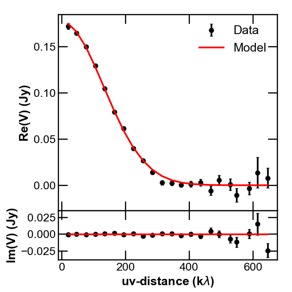
Second, the so called uv-plot which shows the comparison between the visibilities of the bestfit model and the observed ones (bottom right figure). To produce the uv-plot we use the uvplot package, which can be easily installed with pip install uvplot.

# do the uv-plot
# select the bestfit model (here, e.g., the model with median parameters)
bestfit = [np.percentile(samples[:, i], 50) for i in range(ndim)]

f0, sigma, inc, PA, dRA, dDec = bestfit

f0 = 10.**f0        # convert from log to real space

# convert to radians
sigma *= arcsec
Rmin *= arcsec
dR *= arcsec
inc *= deg
PA *= deg
dRA *= arcsec
dDec *= arcsec

f = GaussianProfile(f0, sigma, Rmin, dR, nR)

# compute the visibilities of the bestfit model
vis_mod = g_double.sampleProfile(f, Rmin, dR, nxy, dxy, u, v,
                                 inc=inc, PA=PA, dRA=dRA, dDec=dDec)

from uvplot import UVTable

uvbin_size = 30e3     # uv-distance bin, units: wle

# observations uv-plot
uv = UVTable(uvtable=[u*wle, v*wle, Re, Im, w], wle=wle)
uv.apply_phase(-dRA, -dDec)         # center the source on the phase center
uv.deproject(inc, PA)
axes = uv.plot(linestyle='.', color='k', label='Data', uvbin_size=uvbin_size)

# model uv-plot
uv_mod = UVTable(uvtable=[u*wle, v*wle, vis_mod.real, vis_mod.imag, w], wle=wle)
uv_mod.apply_phase(-dRA, -dDec)     # center the source on the phase center
uv_mod.deproject(inc, PA)
uv_mod.plot(axes=axes, linestyle='-', color='r', label='Model', yerr=False, uvbin_size=uvbin_size)

axes[0].figure.savefig("uvplot_example.pdf")

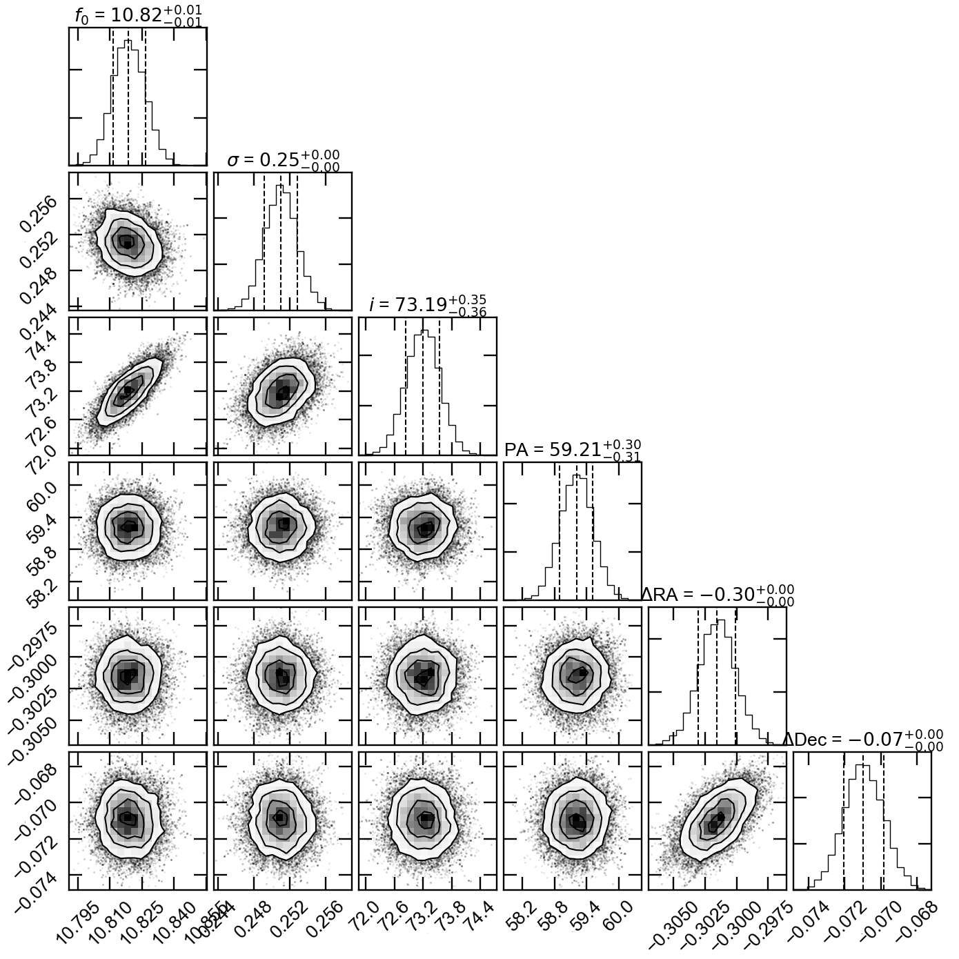
Corner plot showing the marginalised posteriors	Uv-plot showing the deprojected visibilities

7) CPU vs GPU execution

So far we have run galario on the CPU. Running it on a GPU can be done by just changing the import at the beginning:

from galario import double_cuda as g_double

All the rest of the code remains the same!

For more details on the GPU vs CPU execution, see the Cookbook.